Monte Carlo Simulator
A Monte Carlo method simulator web app with custom reporting for re-usable workflows.
The Monte Carlo app is still in development and not production-ready. However, you can play around with it at the link below:
Overview and Usage
montecarlo is an R web app for Monte Carlo simulations using the shiny package.
The goal of the project is to provide a framework for users to develop re-useable simulation workflows, while simultaneously exposing enough underlying R directly to the user for them to incorporate any use case.
Simulation results can be reported as pdf, docx, html, or csv, as well as graphically within the app.
Commercial Monte Carlo simulators such as Crystal Ball cost about $1000 per individual license.
The app allows the user to define aspects of their simulation in several R snippets. For example, one snippet is run once and inherited by all subsequent iterations. Other snippets are executed once per iteration. Others allow for post-simulation data processing, plotting, and other reporting.
The result is a set of R environments defining each trial that was performed. R then inspects the variables these environments to generate a tidy data frame of simulation results. A goal of the project is to make minimal assumptions about the particular use case, so it is possible to do things like include variables in some trials but not others, or to name variables programmatically.
When launched, montecarlo loads a simple sample simulation.

Simulation
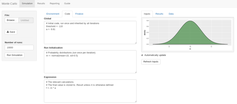
The Simulation tab provides the functionality required to run Monte Carlo simulations.
Loading and saving simulations
A side panel allows for loading and saving of simulation parameters (as JSON).
Scripting the simulation
Subtabs in the Simulation tab provide the primary coding interface for defining the simulation.
The Environment tab is used to load libraries and define helper functions for later use. The intent of this area is for code that is not necessarily specific to the current simulation.
The Code tab contains three code entry textboxes.
The Global textbox is executed once per simulation, and is inherited by all trials.
The Initialization textbox is executed once per trial.
This is a good place to define the random probability distribution variables, as variables defined in this textbox are graphically displayed in the Inputs tab described below.
montecarlo provides functions for generating probability distributions, for example:
normal(mean=0, sd=1)
uniform(min=0, max=1)
# ...
These montecarlo functions are preferred to native code, although any R code can be used to define your probability distributions.
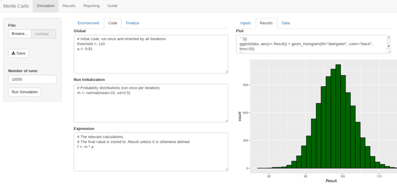
The Expression textbox is for the meat and potatoes of your simulation code.
The last calculation in the Expression textbox will be represented as .Result within the simulation result dataframe (unless otherwise explicitly defined).
The Finalize subtab is run once, after the simulation. The dataframe resulting from the simulation is stored in the variable data, and can be modified or new columns can be added. Additionally, summary variables such as column averages can be defined. These can later be used during reporting.
data_frame(
  x = seq(7.5, 12.5, length=1000),
  m = dnorm(x, mean=10, sd=0.5)
) %>%
ggplot(aes(x=x, ymin=0, ymax=m)) + geom_ribbon(fill="darkgreen", alpha=0.5, color="black")
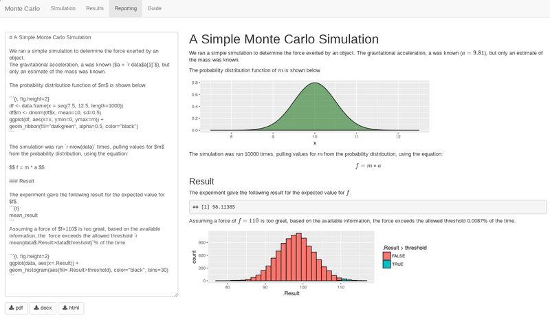
The simulation was run r nrow(data) times, pulling values for $m$ from the probability distribution, using the equation:
$$ f = m * a $$
Result
The experiment gave the following result for the expected value for $f$.
mean_result
Assuming a force of $f=110$ is too great, based on the available information, the force exceeds the allowed threshold r mean(data$.Result>data$threshold)% of the time.
ggplot(data, aes(x=.Result)) + geom_histogram(aes(fill=.Result>threshold), color="black", bins=30)
On the right-hand side of the screen, there are three tabs which provide feedback on the simulation parameters and results. The Inputs tab provides a graphical representation of the probability distribution variables. The Results tab provides an overview of the results. By default, it shows the distribution of the .Result variable, however, the behaviour can be modified using the related code textbox. The data tab provides a method for inspecting the data within the results dataframe.

Results
The results tab provides further ability to review the simulation results. At present, it contains a datatable of the results and the ability to export as csv, however, additional features will be added.
Reporting
The reporting tab allows the user to generate a report using rmarkdown to produce a pdf, docx, or html document.
This allows the user to load a saved Monte Carlo simulation JSON file, tweak the parameters, run a simulation, and generate a final report all from a single app.
The simulation results dataframe is available as the variable data, as well as any variables defined in the Finalize subtab within Simulation.
Download buttons are provided for the various download formats.

Settings
The Settings tab is reserved for settings such as user preferences.
Guide
The Guide tab contains basic guidance for the app.
Installation
The development version of the app can be downloaded or cloned from GitHub (gmyrland/montecarlo).
Prerequisites
There are several dependencies for full feature functionality. Most notably, pdf reporting requires a TeX distribution be installed.
apt-get intall -y texlive texlive-latex-extra
You could also install an alternate distribution such as MikTex on Windows and Mac.
The RStudio IDE also provides many features which make it easy to work with Shiny apps.
Deployment
The app can be deployed in a number of ways, including on a Shiny Server. However, note that one of the design features of the app is to allow the user to script and execute arbitrary R code. As such, it is a bad idea to expose the interface to untrusted users.
Docker
A Dockerfile is provided as a simple method of deployment the app from a Docker container. The generated Docker image includes all dependencies and required packages and serves the app from a containerized Shiny Server.
With docker installed, build the container image and launch as shown below.
# build docker container
docker build -t montecarlo .

# launch docker container
docker run --rm -p 3838:3838 --name montecarlo \
   -v `pwd`:/srv/shiny-server/:ro \
   montecarlo
At this point, you can access the app on at localhost:3838. See rocker-org/shiny documentation for more information about the underlying container image and shiny server deployment in Docker.
Author
Glen Myrland